Random Variables - Distribution and Expectation
Random Variables: Distribution and Expectation
Example: Coin Flips
Recall our setup of a probabilistic experiment as a procedure of drawing a sample from a set of possible values, and assigning a probability for each possible outcome of the experiment. For example, if we toss a fair coin \(n\) times, then there are \(2^n\) possible outcomes, each of which is equally likely and has probability \(2^{-n}\).
Now suppose we want to make a measurement in our experiment. For example, we can ask what is the number of heads in \(n\) coin tosses; call this number \(X\). Of course, \(X\) is not a fixed number, but it depends on the actual sequence of coin flips that we obtain. For example, if \(n = 4\) and we observe the outcome \(\omega = HTHH\), then the number of heads is \(X = 3\); whereas if we observe the outcome \(\omega = HTHT\), then the number of heads is \(X = 2\). In this example of \(n\) coin tosses we only know that \(X\) is an integer between \(0\) and \(n\), but we do not know what its exact value is until we observe which outcome of \(n\) coin flips is realized and count how many heads there are. Because every possible outcome is assigned a probability, the value \(X\) also carries with it a probability for each possible value it can take. The table below lists all the possible values \(X\) can take in the example of \(n = 4\) coin tosses, along with their respective probabilities.
| outcomes \(\omega\) | value of \(X\) (number of heads) | probability |
|---|---|---|
| \(TTTT\) | \(0\) | \(1/16\) |
| \(HTTT, THTT, TTHT, TTTH\) | \(1\) | \(4/16\) |
| \(HHTT, HTHT, HTTH, THHT, THTH, TTHH\) | \(2\) | \(6/16\) |
| \(HHHT, HHTH, HTHH, THHH\) | \(3\) | \(4/16\) |
| \(HHHH\) | \(4\) | \(1/16\) |
Such a value \(X\) that depends on the outcome of the probabilistic experiment is called a random variable (or r.v.). As we see from the example above, \(X\) does not have a definitive value, but instead only has a probability distribution over the set of possible values \(X\) can take, which is why it is called random. So the question “What is the number of heads in \(n\) coin tosses?” does not exactly make sense because the answer \(X\) is a random variable. But the question “What is the typical number of heads in \(n\) coin tosses?” makes sense: it is asking what is the average value of \(X\) (the number of heads) if we repeat the experiment of tossing \(n\) coins multiple times. This average value is called the expectation of \(X\), and is one of the most useful summary (also called statistics) of an experiment.
Example: Permutations
Before we formalize all these notions, let us consider another example to enforce our conceptual understanding of a random variable. Suppose we collect the homeworks of \(n\) students, randomly shuffle them, and return them to the students. How many students receive their own homework?
Here the probability space consists of all \(n!\) permutations of the homeworks, each with equal probability \(1/n!\). If we label the homeworks as \(1,2,\dots,n\), then each sample point is a permutation \(\pi = (\pi_1,\dots,\pi_n)\) where \(\pi_i\) is the homework that is returned to the \(i\)-th student. Note that \(\pi_1,\dots,\pi_n \in \{1,2,\dots,n\}\) are all distinct, so each element in \(\{1,\dots,n\}\) appears exactly once in the permutation \(\pi\).
In this setting, the \(i\)-th student receives her own homework if and only if \(\pi_i = i\). Then the question “How many students receive their own homework?” translates into the question of how many indices \(i\)’s satisfy \(\pi_i = i\). These are known as fixed points of the permutation. As in the coin flipping case above, our question does not have a simple numerical answer (such as \(4\)), because the number depends on the particular permutation we choose (i.e., on the sample point). Let’s call the number of fixed points \(X\), which is a random variable.
To illustrate the idea concretely, let’s consider the example \(n = 3\). The following table gives a complete listing of the sample space (of size \(3!=6\)), together with the corresponding value of \(X\) for each sample point. Here we see that \(X\) takes on values \(0\), \(1\), or \(3\), depending on the sample point. You should check that you agree with this table.
| permutation \(\pi\) | value of \(X\) (number of fixed points) |
|---|---|
| \((1, 2, 3)\) | \(3\) |
| \((1, 3, 2)\) | \(1\) |
| \((2, 1, 3)\) | \(1\) |
| \((2, 3, 1)\) | \(0\) |
| \((3, 1, 2)\) | \(0\) |
| \((3, 2, 1)\) | \(1\) |
Random Variables
Let us formalize the concepts discussed above.
Definition 1 (Random Variable)
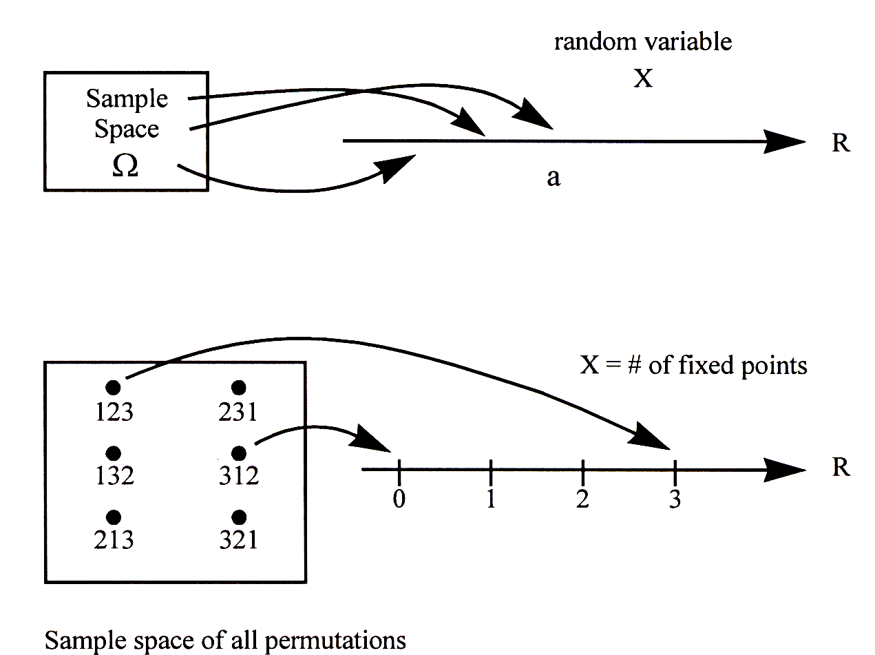
A random variable \(X\) on a sample space \(\Omega\) is a function \(X : \Omega \to \mathbb{R}\) that assigns to each sample point \(\omega\in\Omega\) a real number \(X(\omega)\).
Until further notice, we will restrict out attention to random variables that are discrete, i.e., they take values in a range that is finite or countably infinite. This means even though we define \(X\) to map \(\Omega\) to \(\mathbb{R}\), the actual set of values \(\{X(\omega) : \omega \in \Omega\}\) that \(X\) takes is a discrete subset of \(\mathbb{R}\).
A random variable can be visualized in general by the picture in Figure 1.1 Note that the term “random variable” is really something of a misnomer: it is a function so there is nothing random about it and it is definitely not a variable! What is random is which sample point of the experiment is realized and hence the value that the random variable maps the sample point to.

Figure 1: Visualization of how a random variable is defined on the sample space.
Distribution
When we introduced the basic probability space in Note 13, we defined two things:
the sample space \(\Omega\) consisting of all the possible outcomes (sample points) of the experiment;
the probability of each of the sample points.
Analogously, there are two things important about any random variable:
the set of values that it can take;
the probabilities with which it takes on the values.
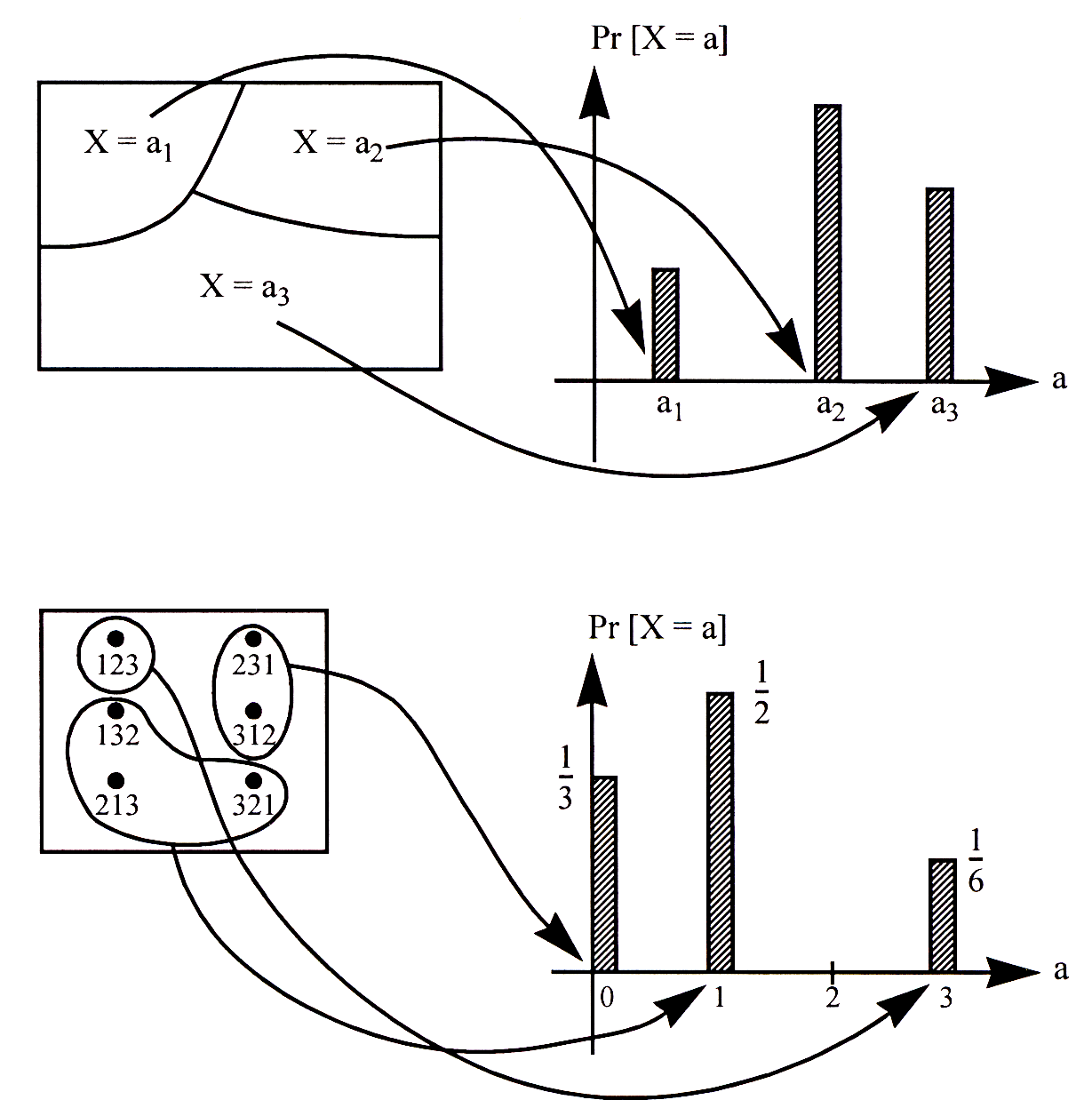
Since a random variable is defined on a probability space, we can calculate these probabilities given the probabilities of the sample points. Let \(a\) be any number in the range of a random variable \(X\). Then the set \[\{\omega\in\Omega:X(\omega)=a\}\] is an event in the sample space (simply because it is a subset of \(\Omega\)). We usually abbreviate this event to simply “\(X=a\)”. Since \(X=a\) is an event, we can talk about its probability, \({\mathbb{P}}[X=a]\). The collection of these probabilities, for all possible values of \(a\), is known as the distribution of the random variable \(X\).
Definition 2 (Distribution)
The distribution of a discrete random variable \(X\) is the collection of values \(\{(a,{\mathbb{P}}[X=a]):a\in\mathcal{A}\}\), where \(\mathcal{A}\) is the set of all possible values taken by \(X\).
Thus, the distribution of the random variable \(X\) in our permutation example above is: \[{\mathbb{P}}[X=0]={1\over 3};\qquad{\mathbb{P}}[X=1]={1\over 2};\qquad{\mathbb{P}}[X=3]={1\over 6};\] and \({\mathbb{P}}[X=a]=0\) for all other values of \(a\).
The distribution of a random variable can be visualized as a bar diagram, shown in Figure 2. The \(x\)-axis represents the values that the random variable can take on. The height of the bar at a value \(a\) is the probability \({\mathbb{P}}[X=a]\). Each of these probabilities can be computed by looking at the probability of the corresponding event in the sample space.

Figure 2: Visualization of how the distribution of a random variable is defined.
Note that the collection of events \(X=a\), \(a \in \mathcal{A}\), satisfy two important properties:
Any two events \(X=a_1\) and \(X= a_2\) with \(a_1 \not = a_2\) are disjoint.
The union of all these events is equal to the entire sample space \(\Omega\).
The collection of events thus form a partition of the sample space (see Figure 2). Both properties follow directly from the fact that \(X\) is a function defined on \(\Omega\), i.e., \(X\) assigns a unique value to each and every possible sample point in \(\Omega\). As a consequence, the sum of the probabilities \({\mathbb{P}}[X=a]\) over all possible values of \(a\) is exactly \(1\). So when we sum up the probabilities of the events \(X=a\), we are really summing up the probabilities of all the sample points.
Example: The Binomial Distribution
Let’s return to our coin tossing example above, where we defined our random variable \(X\) to be the number of heads. More formally, consider the random experiment consisting of \(n\) independent tosses of a biased coin which lands on heads with probability \(p\). Each sample point \(\omega\) is a sequence of tosses. \(X(\omega)\) is defined to be the number of heads in \(\omega\). For example, when \(n = 3\), \(X(THH) = 2\).
To compute the distribution of \(X\), we first enumerate the possible values \(X\) can take on. They are simply \(0, 1, \ldots, n\). Then we compute the probability of each event \(X=i\) for \(i =0, 1, \ldots, n\). The probability of the event \(X=i\) is the sum of the probabilities of all the sample points with exactly \(i\) heads (for example, if \(n=3\) and \(i=2\), there would be three such sample points \(\{HHT, HTH, THH\}\)). Any such sample point has a probability \(p^i(1-p)^{n-i}\), since the coin flips are independent. There are exactly \(n \choose i\) of these sample points. So \[{\mathbb{P}}[X=i] = {n \choose i} p^i(1-p)^{n-i} \qquad \text{ for } ~ i =0,1, \ldots, n.\]
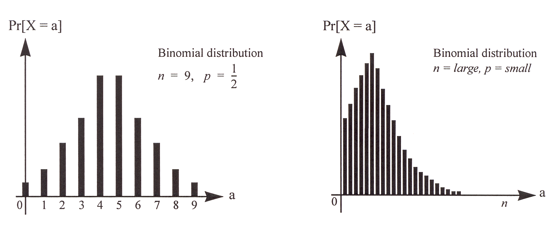
This distribution, called the binomial distribution, is one of the most important distributions in probability. A random variable with this distribution is called a binomial random variable, written as \[X \sim {\operatorname{Bin}}(n,p)\] An example of a binomial distribution is shown in Figure 3. Notice that due to the properties of \(X\) mentioned above, it must be the case that \(\sum_{i=0}^{n}{\mathbb{P}}[X=i] = 1\), which implies that \(\sum_{i=0}^{n}{n \choose i}p^i(1-p)^{n-i} = 1\). This provides a probabilistic proof of the Binomial Theorem!

Figure 3: The binomial distributions for two choices of \((n,p)\).
Although we define the binomial distribution in terms of an experiment involving tossing coins, this distribution is useful for modeling many real-world problems. Consider for example the error correction problem studied in Note 9. Recall that we wanted to encode \(n\) packets into \(n+k\) packets such that the recipient can reconstruct the original \(n\) packets from any \(n\) packets received. But in practice, the number of packet losses is random, so how do we choose \(k\), the amount of redundancy? If we model each packet getting lost with probability \(p\) and the losses are independent, then if we transmit \(n+k\) packets, the number of packets received is a random variable \(X\) with binomial distribution: \(X \sim {\operatorname{Bin}}(n+k,1-p)\) (we are tossing a coin \(n+k\) times, and each coin turns out to be a head (packet received) with probability \(1-p\)). So the probability of successfully decoding the original data is: \[{\mathbb{P}}[X \ge n] ~=~ \sum_{i=n}^{n+k} {\mathbb{P}}[X = i] ~=~ \sum_{i=n}^{n+k} {n+k \choose i} (1-p)^i p^{n+k-i}.\] Given fixed \(n\) and \(p\), we can choose \(k\) such that this probability is no less than, say, \(0.99\).
Expectation
The distribution of a r.v. contains all the probabilistic information about the r.v. In most applications, however, the complete distribution of a r.v. is very hard to calculate. For example, consider the homework permutation example with \(n = 20\). In principle, we’d have to enumerate \(20!\approx 2.4\times10^{18}\) sample points, compute the value of \(X\) at each one, and count the number of points at which \(X\) takes on each of its possible values! (Though in practice we could streamline this calculation a bit.) Moreover, even when we can compute the complete distribution of a r.v., it is often not very informative.
For these reasons, we seek to compress the distribution into a more compact, convenient form that is also easier to compute. The most widely used such form is the expectation (or mean or average) of the r.v.
Definition 3 (Expectation)
The expectation of a discrete random variable \(X\) is defined as \[{\mathbb{E}}[X]=\sum_{a\in\mathcal{A}} a\times{\mathbb{P}}[X=a],\] where the sum is over all possible values taken by the r.v.
For our simpler permutation example with only \(3\) students, the expectation is \[{\mathbb{E}}[X]=\left( 0\times{1\over 3}\right) + \left( 1\times{1\over 2}\right) + \left( 3\times{1\over 6}\right) = 0+{1\over 2}+{1\over 2} = 1.\] That is, the expected number of fixed points in a permutation of three items is exactly \(1\).
The expectation can be seen in some sense as a “typical” value of the r.v. (though note that it may not actually be a value that the r.v. ever takes on). The question of how typical the expectation is for a given r.v. is a very important one that we shall return to in a later lecture.
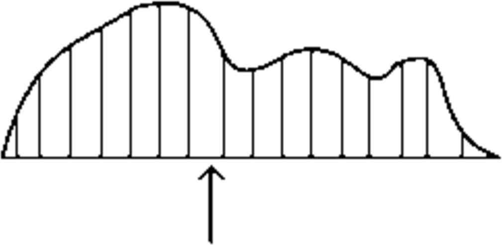
Here is a physical interpretation of the expectation of a random variable: imagine carving out a wooden cutout figure of the probability distribution as in Figure 4. Then the expected value of the distribution is the balance point (directly below the center of gravity) of this object.

Figure 4: Physical interpretation of expected value as the balance point.
Examples
Single die. Throw one fair die. Let \(X\) be the number that comes up. Then \(X\) takes on values \(1,2,\ldots,6\) each with probability \(1/6\), so \[{\mathbb{E}}[X]={1\over 6}(1+2+3+4+5+6)={{21}\over 6} = {7\over 2}.\] Note that \(X\) never actually takes on its expected value \(7/2\).
Two dice. Throw two fair dice. Let \(X\) be the sum of their scores. Then the distribution of \(X\) is: \[\begin{array}{|c|ccccccccccc|} \hline a & 2 & 3 & 4 & 5 & 6 & 7 & 8 & 9 & 10 & 11 & 12 \\ \hline {\mathbb{P}}[X = a] & 1/36 & 1/18 & 1/12 & 1/9 & 5/36 & 1/6 & 5/36 & 1/9 & 1/12 & 1/18 & 1/36 \\ \hline \end{array}\] The expectation is therefore \[{\mathbb{E}}[X]=\left(2\times{1\over{36}}\right)+\left(3\times{1\over{18}}\right) +\left(4\times{1\over{12}}\right)+\cdots+\left(12\times{1\over{36}}\right)=7.\]
Roulette. A roulette wheel is spun (recall that a roulette wheel has \(38\) slots: the numbers \(1,2,\ldots,36\), half of which are red and half black, plus \(0\) and \(00\), which are green). You bet \(\$1\) on Black. If a black number comes up, you receive your stake plus \(\$1\); otherwise you lose your stake. Let \(X\) be your net winnings in one game. Then \(X\) can take on the values \(+1\) and \(-1\), and \({\mathbb{P}}[X=1]=18/38\), \({\mathbb{P}}[X=-1]=20/38\). Thus, \[{\mathbb{E}}[X] = \left(1\times{{18}\over{38}}\right) + \left(-1\times{{20}\over{38}}\right) = -{1\over{19}};\] i.e., you expect to lose about a nickel per game. Notice how the zeros tip the balance in favor of the casino!
Linearity of Expectation
So far, we’ve computed expectations by brute force: i.e., we have written down the whole distribution and then added up the contributions for all possible values of the r.v. The real power of expectations is that in many real-life examples they can be computed much more easily using a simple shortcut. The shortcut is the following:
Theorem 1
For any two random variables \(X\) and \(Y\) on the same probability space, we have \[{\mathbb{E}}[X+Y]={\mathbb{E}}[X]+{\mathbb{E}}[Y].\] Also, for any constant \(c\), we have \[{\mathbb{E}}[cX] = c{\mathbb{E}}[X].\]
Proof. To make the proof easier, we will first rewrite the definition of expectation in a more convenient form. Recall from Definition 3 that \[{\mathbb{E}}[X]=\sum_{a\in\mathcal{A}} a\times{\mathbb{P}}[X=a].\] Let’s look at one term \(a\times{\mathbb{P}}[X=a]\) in the above sum. Notice that \({\mathbb{P}}[X=a]\), by definition, is the sum of \({\mathbb{P}}[\omega]\) over those sample points \(\omega\) for which \(X(\omega)=a\). And we know that every sample point \(\omega\in\Omega\) is in exactly one of these events \(X=a\). This means we can write out the above definition in a more long-winded form as \[ {\mathbb{E}}[X]=\sum_{\omega\in\Omega} X(\omega)\times{\mathbb{P}}[\omega].\](1) This equivalent definition of expectation will make the present proof much easier (though it is usually less convenient for actual calculations).
Now let’s write out \({\mathbb{E}}[X+Y]\) using Equation 1: \[\begin{aligned} {\mathbb{E}}[X+Y]&=\sum_{\omega\in\Omega} (X+Y)(\omega)\times{\mathbb{P}}[\omega]\cr &=\sum_{\omega\in\Omega} (X(\omega)+Y(\omega))\times{\mathbb{P}}[\omega]\cr &=\sum_{\omega\in\Omega} \Bigl(X(\omega)\times{\mathbb{P}}[\omega]\Bigr) + \sum_{\omega\in\Omega} \Bigl(Y(\omega)\times{\mathbb{P}}[\omega]\Bigr)\cr &= {\mathbb{E}}[X] + {\mathbb{E}}[Y].\end{aligned}\] In the last step, we used Equation 1 twice.
This completes the proof of the first equality. The proof of the second equality is much simpler and is left as an exercise. \(\square\)
Theorem 1 is very powerful: it says that the expectation of a sum of r.v.’s is the sum of their expectations, with no assumptions about the r.v.'s. We can use Theorem 1 to conclude things like \({\mathbb{E}}[3X-5Y]=3{\mathbb{E}}[X]-5{\mathbb{E}}[Y]\). This property is known as linearity of expectation.
Important caveat: Theorem 1 does not say that \({\mathbb{E}}[XY]={\mathbb{E}}[X]{\mathbb{E}}[Y]\), or that \({\mathbb{E}}[1/X]=1/{\mathbb{E}}[X]\), etc. These claims are not true in general. It is only sums and differences and constant multiples of random variables that behave so nicely.
Examples
Now let’s see some examples of Theorem 1 in action.
Two dice again. Here’s a much less painful way of computing \({\mathbb{E}}[X]\), where \(X\) is the sum of the scores of the two dice. Note that \(X=X_1+X_2\), where \(X_i\) is the score on die \(i\). We know from example 1 above that \({\mathbb{E}}[X_1]={\mathbb{E}}[X_2]=7/2\). So by Theorem 1 we have \({\mathbb{E}}[X]={\mathbb{E}}[X_1]+{\mathbb{E}}[X_2]=7\).
More roulette. Suppose we play the above roulette game not once, but \(1000\) times. Let \(X\) be our expected net winnings. Then \(X=X_1+X_2+\cdots+X_{1000}\), where \(X_i\) is our net winnings in the \(i\)th play. We know from earlier that \({\mathbb{E}}[X_i]=-1/19\) for each \(i\). Therefore, by Theorem 1, \({\mathbb{E}}[X]={\mathbb{E}}[X_1]+{\mathbb{E}}[X_2]+\cdots+{\mathbb{E}}[X_{1000}]=1000\times(-1/19) =-1000/19\approx -53\). So if you play \(1000\) games, you expect to lose about \(\$53\).
Homeworks. Let’s go back to our homework permutation example with \(n = 20\) students. Recall that the r.v. \(X\) is the number of students who receive their own homework after shuffling (or equivalently, the number of fixed points). To take advantage of Theorem 1, we need to write \(X\) as the sum of simpler r.v.’s. But since \(X\) counts the number of times something happens, we can write it as a sum using the following trick: \[ X=X_1+X_2+\cdots+X_{20},\qquad\text{where } X_i=\begin{cases} 1 & \text{if student $i$ gets her own hw}; \\ 0 & \text{otherwise}. \end{cases}\](2) [You should think about this equation for a moment. Remember that all the \(X\)’s are random variables. What does an equation involving random variables mean? What we mean is that, at every sample point \(\omega\), we have \(X(\omega)=X_1(\omega)+X_2(\omega)+\cdots+X_{20}(\omega)\). Why is this true?]
A \(\{0,1\}\)-valued random variable such as \(X_i\) is called an indicator random variable of the corresponding event (in this case, the event that student \(i\) gets her own hw). For indicator r.v.’s, the expectation is particularly easy to calculate. Namely, \[{\mathbb{E}}[X_i]=(0\times{\mathbb{P}}[X_i=0]) + (1\times{\mathbb{P}}[X_i=1]) = {\mathbb{P}}[X_i=1].\] But in our case, we have \[{\mathbb{P}}[X_i=1] = {\mathbb{P}}[\text{student $i$ gets her own hw}] = {1\over{20}}.\] Now we can apply Theorem 1 to Equation 2, to get \[{\mathbb{E}}[X]={\mathbb{E}}[X_1]+{\mathbb{E}}[X_2]+\cdots+{\mathbb{E}}[X_{20}]=20\times \frac{1}{20} = 1.\] So we see that the expected number of students who get their own homeworks in a class of size \(20\) is \(1\). But this is exactly the same answer as we got for a class of size \(3\)! And indeed, we can easily see from the above calculation that we would get \({\mathbb{E}}[X]=1\) for any class size \(n\): this is because we can write \(X=X_1+X_2+\cdots+X_n\), and \({\mathbb{E}}[X_i]=1/n\) for each \(i\).
So the expected number of fixed points in a random permutation of \(n\) items is always \(1\), regardless of \(n\). Amazing, but true.
Coin tosses. Toss a fair coin \(100\) times. Let the r.v. \(X\) be the number of Heads. As in the previous example, to take advantage of Theorem 1 we write \[X=X_1+X_2+\cdots+X_{100},\] where \(X_i\) is the indicator r.v. of the event that the \(i\)-th toss is Heads. Since the coin is fair, we have \[{\mathbb{E}}[X_i]={\mathbb{P}}[X_i=1]={\mathbb{P}}[\text{$i$-th toss is Heads}]=\frac{1}{2}.\] Using Theorem 1, we therefore get \[{\mathbb{E}}[X] = \sum_{i=1}^{100} \frac{1}{2} = 100\times \frac{1}{2} = 50.\] More generally, the expected number of Heads in \(n\) tosses of a fair coin is \(n/2\). And in \(n\) tosses of a biased coin with Heads probability \(p\), it is \(np\) (why?). So the expectation of a binomial r.v. \(X \sim {\operatorname{Bin}}(n,p)\) is equal to \(np\). Note that it would have been harder to reach the same conclusion by computing this directly from definition of expectation.
Balls and bins. Throw \(m\) balls into \(n\) bins. Let the r.v. \(X\) be the number of balls that land in the first bin. Then \(X\) behaves exactly like the number of Heads in \(m\) tosses of a biased coin, with Heads probability \(1/n\) (why?). So we get \({\mathbb{E}}[X]=m/n\).
In the special case \(m=n\), the expected number of balls in any bin is \(1\). If we wanted to compute this directly from the distribution of \(X\), we’d get into a messy calculation involving binomial coefficients.
Here’s another example on the same sample space. Let the r.v. \(Y\) be the number of empty bins. The distribution of \(Y\) is horrible to contemplate: to get a feel for this, you might like to write it down for \(m=n=3\) (\(3\) balls, \(3\) bins). However, computing the expectation \({\mathbb{E}}[Y]\) is easy using Theorem 1. As usual, let’s write \[ Y=Y_1+Y_2+\cdots+Y_n,\](3) where \(Y_i\) is the indicator r.v. of the event “bin \(i\) is empty”. Again as usual, the expectation of \(Y_i\) is easy: \[{\mathbb{E}}[Y_i] = {\mathbb{P}}[Y_i=1] = {\mathbb{P}}[\text{bin $i$ is empty}] = \left(1-{1\over n}\right)^m;\] recall that we computed this probability (quite easily) in an earlier lecture. Applying Theorem 1 to Equation 3 we therefore have \[{\mathbb{E}}[Y] = \sum_{i=1}^n{\mathbb{E}}[Y_i]=n\left(1-{1\over n}\right)^m,\] a very simple formula, very easily derived.
Let’s see how it behaves in the special case \(m=n\) (same number of balls as bins). In this case we get \({\mathbb{E}}[Y]=n(1-1/n)^n\). Now the quantity \((1-1/n)^n\) can be approximated (for large enough values of \(n\)) by the number \(1/e\).2 So we see that \[{\mathbb{E}}[Y]\to{n\over{e}}\approx 0.368n\quad\text{as $n\to\infty$}.\]
The bottom line is that, if we throw (say) \(1000\) balls into \(1000\) bins, the expected number of empty bins is about \(368\).
The figures in this note are inspired by figures in Chapter 2 of “Introduction to Probability” by D. Bertsekas and J. Tsitsiklis.↩
More generally, it is a standard fact that for any constant \(c\), \[\left(1+\frac{c}{n}\right)^n\to e^c\quad\text{as $n\to\infty$}.\] We just used this fact in the special case \(c=-1\). The approximation is actually very good even for quite small values of \(n\) — try it yourself! For example, for \(n=20\) we already get \((1-1/n)^n=0.358\), which is very close to \(1/e=0.367\ldots\). The approximation gets better and better for larger \(n\).↩