Markov Chains
Finite Markov Chains
These notes explain the theory of finite Markov chains. For CS 70, we do not cover the proofs that are discussed in Appendix 2.
Introduction
Markov chains are models of random motion in a finite or countable set. These models are powerful because they capture a vast array of systems that we encounter in applications. Yet, the models are simple in that many of their properties can often be determined using elementary matrix algebra. In this course, we limit the discussion to the case of finite Markov chains, i.e., motions in a finite set.
Imagine the following scenario. You flip a fair coin until you get two consecutive ‘heads’. How many times do you have to flip the coin, on average? You roll a balanced six-sided die until the sum of the last two rolls is \(8\). How many times do you have to roll the die, on average?
As another example, say that you play a game of ‘heads or tails’ using a biased coin that yields ‘heads’ with probability \(0.48\). You start with \(\$10\). At each step, if the flip yields ‘heads’, you earn \(\$1\). Otherwise, you lose \(\$1\). What is the probability that you reach \(\$100\) before \(\$0\)? How long does it take until you reach either \(\$100\) or \(\$0\)?
You try to go up a ladder that has \(20\) rungs. At each time step, you succeed in going up by one rung with probability \(0.9\). Otherwise, you fall back to the ground. How many time steps does it take you to reach the top of the ladder, on average?
You look at a web page, then select randomly one of the links on that page, with equal probabilities. You then repeat on the next page you visit, and so on. As you keep browsing the web in that way, what fraction of the time do you open a given page? How long does it take until you reach a particular page? How likely is it that you visit a given page before another given page?
These questions can be answered using the methods of Markov chains, as we explain in these notes.
A First Example
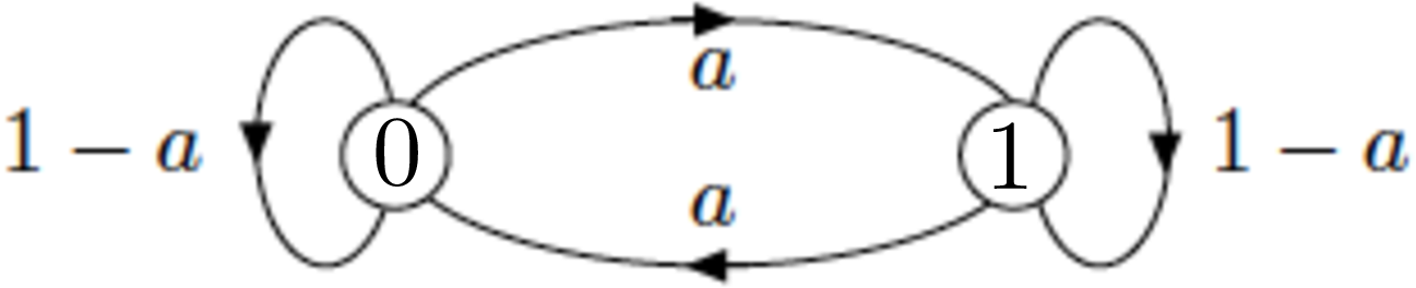
Figure 1: A simple Markov chain.
Figure 1 illustrates a simple Markov chain. It describe a random motion in the set \(\{0, 1\}\). The position at time \(n = 0, 1, 2, \ldots\) is \(X_n \in \{0, 1\}\). We call \(X_n\) the state of the Markov chain at step (or time) \(n\). The set \(\{0, 1\}\) is the state space, i.e., the set of possible values of the state. The motion, i.e., the time evolution, of \(X_n\) follows the following rules. One is given a number \(a \in [0, 1]\) and two nonnegative numbers \(\pi_0(0)\) and \(\pi_0(1)\) that add up to \(1\). Then, \[ {\mathbb{P}}[X_0 = 0] = \pi_0(0) \text{ and } {\mathbb{P}}[X_0 = 1] = \pi_0(1).\](1) That is, the initial state \(X_0\) is equal to \(0\) with probability \(\pi_0(0)\), otherwise it is \(1\). Then for \(n \geq 0\), \[\begin{aligned} {\mathbb{P}}[X_{n+1} = 0 \mid X_n = 0, X_{n-1}, \ldots, X_0] &= 1 - a \\ {\mathbb{P}}[X_{n+1} = 1 \mid X_n = 0, X_{n-1}, \ldots, X_0] &= a \\ {\mathbb{P}}[X_{n+1} = 0 \mid X_n = 1, X_{n-1}, \ldots, X_0] &= a \\ {\mathbb{P}}[X_{n+1} = 1 \mid X_n = 1, X_{n-1}, \ldots, X_0] &= 1 - a. \end{aligned}\](2) Figure 1 summarizes the rules in Equation 2. These rules specify the transition probabilities of the Markov chain. The first two rules specify that if the Markov chain is in state \(0\) at step \(n\), then at the next step it stays in state \(0\) with probability \(1 - a\) and it moves to state \(1\) with probability \(a\), independently of what happened in the previous steps. Thus, the Markov chain may have been in state \(0\) for a long time prior to step \(n\), or it may have just moved into state \(0\), but the probability of staying in state \(0\) one more step is \(1 - a\) in those different cases. The last two rules are similar. Figure 1 is called the state transition diagram of the Markov chain. It captures the transition probabilities in a graphical form.
In a sense, the Markov chain is amnesic: at step \(n\), it forgets what it did before getting to the current state and its future steps only depend on that current state. Here is one way to think of the rules of motion. When the Markov chain gets to state \(0\), it flips a coin. If the outcome is \(H\), which occurs with probability \(a\), then it goes to state \(1\); otherwise, it stays in state \(0\) one more step. The situation is similar when the Markov chain gets to state \(1\).
We define the transition probability matrix \(P\) by \(P(0, 0) = 1 - a, P(0, 1) = a, P(1, 0) = a, P(1, 1) = 1 - a.\) That is \[P = \begin{bmatrix} 1 - a & a \\ a & 1 - a \end{bmatrix} .\] Hence, \[{\mathbb{P}}[ X_{n+1} = j \mid X_n = i, X_{n-1}, \ldots , X_0] = P(i, j), \text{ for } n \geq 0 \text{ and } i, j \in \{0, 1\}.\]
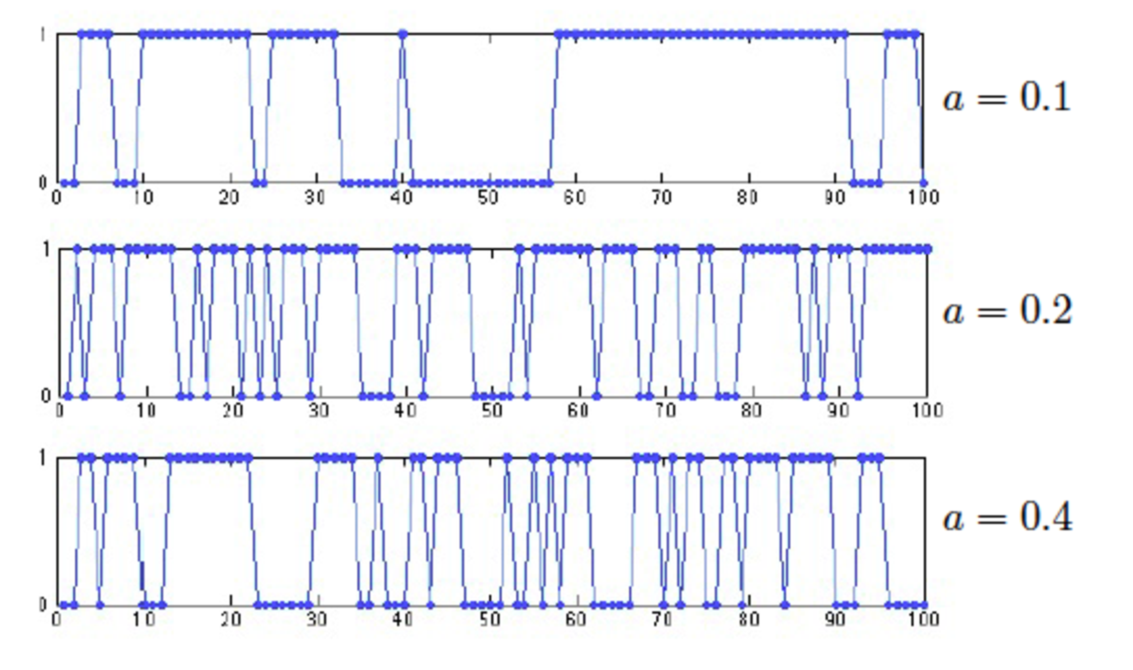
Figure 2: Simulations of the two-state Markov chain.
Figure 2 shows some simulations of the Markov chain with different values of \(a\). When \(a = 0.1\), it is unlikely that the state of the Markov chain changes in one step. As the figure shows, the Markov chain spends many steps in one state before switching. For larger values of \(a\), the state of the Markov chain changes more frequently. Note that, by symmetry, over the long term the Markov chain spends half of the time in each state.
A Second Example
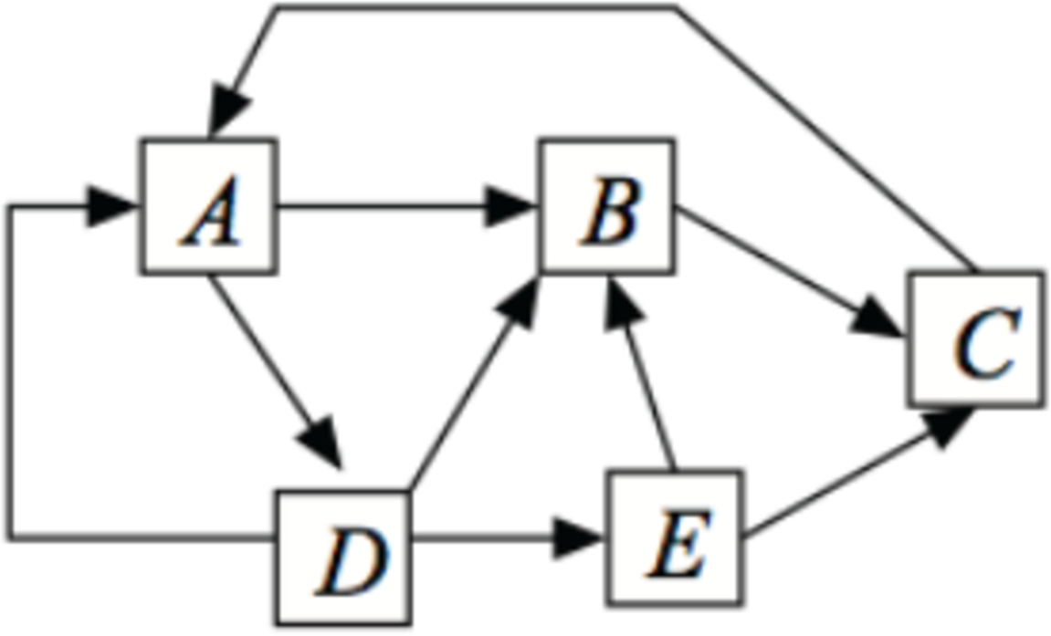
Figure 3: A five-state Markov chain. The outgoing arrows are equally likely.
Figure 3 shows the state transition diagram of a small web browsing experiment. Each state in the figure represents a web page. The arrows out of a state correspond to links on the page that point to other pages. The transition probabilities are not indicated on the figure, but the model is that each outgoing link is equally likely. The figure corresponds to the following probability transition matrix: \[P = \begin{bmatrix} 0 & 1/2 & 0 & 1/2 & 0 \\ 0 & 0 & 1 & 0 & 0 \\ 1 & 0 & 0 & 0 & 0 \\ 1/3 & 1/3 & 0 & 0 & 1/3 \\ 0 & 1/2 & 1/2 & 0 & 0 \\ \end{bmatrix} .\]
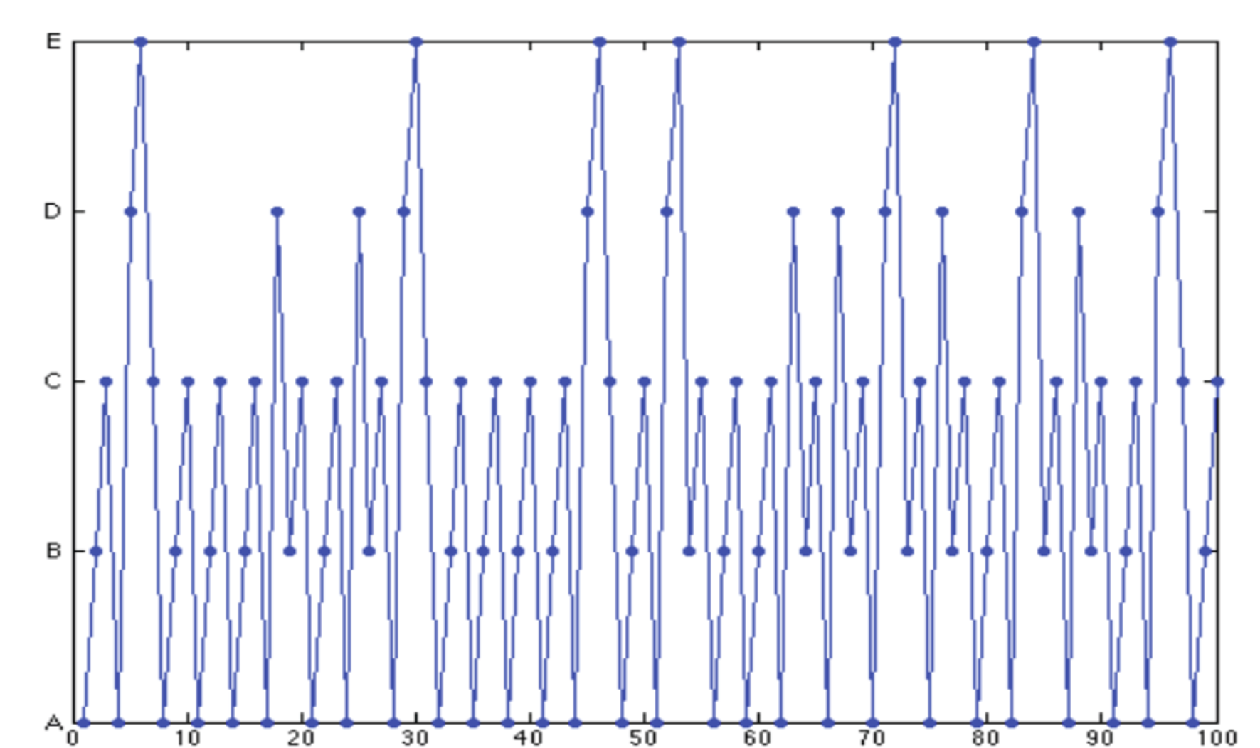
Figure 4: Simulation of the five-state Markov chain.
Figure 4 shows a simulation of the five-state Markov chain.
Finite Markov Chains
One defines a general finite Markov chain as follows. The state space is \({\cal X} = \{1, 2, \ldots, K\}\) for some finite \(K\). The transition probability matrix \(P\) is a \(K \times K\) matrix such that \[P(i, j) \geq 0, \forall i, j \in {\cal X}\] and \[\sum_{j = 1}^K P(i, j) = 1, \forall i \in {\cal X}.\] The initial distribution is a vector \(\pi_0 = \{\pi_0(i), i \in {\cal X}\}\) where \(\pi_0(i) \geq 0\) for all \(i \in {\cal X}\) and \(\sum_{i \in {\cal X}} \pi_0(i) = 1\).
One then defines the random sequence \(\{X_n, n = 0, 1, 2, \ldots \}\) by \[\begin{aligned} {\mathbb{P}}[X_0 = i] &= \pi_0(i), i \in {\cal X} \\ {\mathbb{P}}[X_{n+1} = j \mid X_n = i, X_{n-1}, \ldots, X_0] &= P(i, j), \forall n \geq 0, \forall i, j \in {\cal X} . \end{aligned}\]
Note that \[\begin{aligned} &{\mathbb{P}}[X_0 = i_0, X_1 = i_1, \ldots, X_n = i_n] \\ &\qquad = {\mathbb{P}}[X_0 = i_0] {\mathbb{P}}[X_1 = i_1 \mid X_0 = i_0] {\mathbb{P}}[X_2 = i_2 \mid X_0 = i_0, X_1 = i_1 ] \cdots {\mathbb{P}}[X_n = i_n \mid X_0 = i_0, \ldots, X_{n-1} = i_{n-1}] \\ &\qquad = \pi_0(i_0) P(i_0, i_1) \cdots P(i_{n-1}, i_n).\end{aligned}\]
Consequently, \[\begin{aligned} {\mathbb{P}}[X_n = i_n] &= \sum_{i_0, \dotsc, i_{n-1}} {\mathbb{P}}[X_0 = i_0, X_1 = i_1, \ldots, X_n = i_n] \\ & = \sum_{i_0, \dotsc, i_{n-1}} \pi_0(i_0) P(i_0, i_1) \cdots P(i_{n-1}, i_n) \\ & = \pi_0 P^n (i_n)\end{aligned}\] where the last expression is component \(i_n\) of the product of the row vector \(\pi_0\) times the \(n\)-th power of the matrix \(P\).
Thus, if we designate by \(\pi_n\) the distribution of \(X_n\), so that \({\mathbb{P}}[X_n = i] = \pi_n(i)\), then the last derivation proves the following result.
Theorem 1
One has \[ \pi_n = \pi_0 P^n, n \geq 0.\] In particular, if \(\pi_0(i) = 1\) for some \(i\), then \(\pi_n(j) = P^n(i, j) = {\mathbb{P}}[X_n = j \mid X_0 = i]\).
For the two-state Markov chain, one can verify that \[ P^n = \begin{bmatrix} 1 - a & a \\ a & 1 - a \end{bmatrix} ^n = \begin{bmatrix} 1/2 + (1/2)(1 - 2a)^n & 1/2 - (1/2)(1 - 2a)^n \\ 1/2 - (1/2)(1 - 2a)^n & 1/2 + (1/2)(1 - 2a)^n \end{bmatrix} .\] Note that if \(0 < a < 1\), \[P^n \to \begin{bmatrix} 1/2 & 1/2 \\ 1/2 & 1/2 \end{bmatrix} , \text{ as } n \to \infty.\](3) Consequently, for \(0 < a < 1\), one has \(\pi_n = \pi_0 P^n \to \begin{bmatrix}1/2 & 1/2\end{bmatrix}\) as \(n \to \infty\).
Balance Equations
The following definition introduces the important notion of invariant distribution.
Definition 1
A distribution \(\pi\) is invariant for the transition probability matrix \(P\) if it satisfies the following balance equations: \[ \pi = \pi P.\](4)
The relevance of this definition is stated in the next result.
Theorem 2
One has \[\pi_n = \pi_0, \forall n \geq 0\] if and only if \(\pi_0\) is invariant.
Proof. If \(\pi_n = \pi_0\) for all \(n \geq 0\), then \(\pi_0 = \pi_1 = \pi_0 P\), so that \(\pi_0\) satisfies Equation 4 and is thus invariant.
If \(\pi_0 P = \pi_0\), then \(\pi_1 = \pi_0 P = \pi_0\). Also, if \(\pi_n = \pi_0\), then \(\pi_{n+1} = \pi_n P = \pi_0 P = \pi_0\). \(\square\)
For instance, in the case of the two-state Markov chain, the balance equations are \[\begin{aligned} \pi(0)& = \pi(0) (1 - a) + \pi(1) a \\ \pi(1)& = \pi(0)a + \pi(1) (1 - a).\end{aligned}\] Each of these two equations is equivalent to \[\pi(0) = \pi(1).\] Thus, the two equations are redundant. If we add the condition that the components of \(\pi\) add up to one, we find that the only solution is \(\begin{bmatrix} \pi(0) & \pi(1) \end{bmatrix} = \begin{bmatrix} 1/2 & 1/2 \end{bmatrix}\), which is not surprising in view of symmetry.
For the five-state Markov chain, the balance equations are \[\begin{bmatrix} \pi(A) & \pi(B) & \pi(C) & \pi(D) & \pi(E) \end{bmatrix} = \begin{bmatrix} \pi(A) & \pi(B) & \pi(C) & \pi(D) & \pi(E) \end{bmatrix} \begin{bmatrix} 0 & 1/2 & 0 & 1/2 & 0 \\ 0 & 0 & 1 & 0 & 0 \\ 1 & 0 & 0 & 0 & 0 \\ 1/3 & 1/3 & 0 & 0 & 1/3 \\ 0 & 1/2 & 1/2 & 0 & 0 \\ \end{bmatrix} .\] Once again, these five equations in the five unknowns are redundant. They do not determine \(\pi\) uniquely. However, if we add the condition that the components of \(\pi\) add up to one, then we find that the solution is unique and given by (see the appendix for the calculations) \[ \begin{bmatrix} \pi(A) & \pi(B) & \pi(C) & \pi(D) & \pi(E)\end{bmatrix} = \frac{1}{39} \begin{bmatrix} 12 & 9 & 10 & 6 & 2 \end{bmatrix}.\](5) Thus, in this web-browsing examples, page \(A\) is visited most often, then page \(C\), then page \(B\). A Google search would return the pages in order of most frequent visits, i.e., in the order \(A, C, B, D, E\). This ranking of the pages is called PageRank and can be determined by solving the balance equations. (In fact, the actual ranking by Google combines the estimate of \(\pi\) with other factors.)
How many invariant distributions does a Markov chain have? We have seen that for the two examples, the answer was one. However, that is not generally the case. For instance, consider the two-state Markov chain with \(a = 0\) instead of \(0 < a < 1\) as we assumed previously. This Markov chain does not change state. Its transition probability matrix is \(P = I\) where \(I\) denotes the identity matrix. Since \(\pi I = \pi\) for any vector \(\pi\), we see that any distribution is invariant for this Markov chain. This is intuitively clear since the Markov chain does not change state, so that the distribution of the state does not change.
However, we show in Theorem 3 that a simple condition guarantees the uniqueness of the invariant distribution.
Fraction of Time in States
How much time does a Markov chain spend in state \(i\), in the long term? That is, what is the long term fraction of time that \(X_n = i\)? We can write this long term fraction of time as \[\lim_{n \to \infty} \frac{1}{n} \sum_{m= 0}^{n-1} 1\{X_m = i\}.\] To understand this expression, note that \(\sum_{m= 0}^{n-1} 1\{X_m = i\}\) counts the number of steps among steps \(\{0, 1, \ldots, n - 1\}\) that \(X_m = i\). Thus, \(n^{-1} \sum_{m= 0}^{n-1} 1\{X_m = i\}\) is the fraction of time among the first \(n\) steps that \(X_m = i\). By taking the limit, we obtain the long term fraction of time that \(X_m = i\).
To study this long term fraction of time, we need one property: irreducibility.
Definition 2 (Irreducible)
A Markov chain is irreducible if it can go from every state \(i\) to every other state \(j\), possibly in multiple steps.
The two-state Markov chain is irreducible when \(0 < a < 1\), not when \(a = 0\). The Markov chain in Figure 3 is irreducible. Observe that a Markov chain is irreducible if and only if its state transition diagram is a directed graph with a single connected component. In this transition diagram, there is an arrow from state \(i\) to state \(j\) if \(P(i, j) > 0\).
Here is a remarkable result.
Theorem 3
Consider a finite irreducible Markov chain with state space \({\cal X}\) and transition probability matrix \(P\). Then, for any initial distribution \(\pi_0\),1 \[ \lim_{n \to \infty} \frac{1}{n} \sum_{m=0}^{n-1} 1\{X_m = i\} = \pi(i), \forall i \in {\cal X}.\](8) In Equation 8, \(\pi = \{\pi(i), i \in {\cal X}\}\) is an invariant distribution. Consequently, the invariant distribution exists and is unique.
We sketch the proof of the result in the appendix. Here, we outline the main points of the argument. Consider the Markov chain in Figure 3. Assume that \(X_0 = A\) and let \(T(A)\) be the first time after \(0\) that the Markov chain comes back to \(A\). This random time has some mean value \({\mathbb{E}}[T(A)]\). Let \(\pi(A) = 1/{\mathbb{E}}[T(A)]\). Thus, the time between two visits to \(A\) has mean value \({\mathbb{E}}[T(A)]\), so that the fraction of time that the Markov chain is in state \(A\) is \(\pi(A)\). Hence, over a long time \(n\), the Markov chain is in state \(A\) for about \(n \pi(A)\) steps. We define \(\pi(i)\) in the same way for the other states. These fractions of time in the different states must add up to one. Also, we claim that \(\pi\) satisfies the balance equations. To see this, note that over a large number \(n\) of steps, the Markov chain visits \(D\) and then \(A\) about \(n \pi(D) P(D, A)\) times. Indeed, it visits \(D\) about \(n \pi(D)\) times and each of these visits is followed by a visit to \(A\) with probability \(P(D, A)\). Similarly, if visits \(C\) and then \(A\) about \(n \pi(C) P(C, A)\) times. Thus, a general Markov chain visits some state \(j\) and then state \(i\) about \(n \pi(j) P(j, i)\) times in \(n\) steps, for \(j \in {\cal X}\). Now, the total number of visits to \(i\) in \(n\) steps is the total number of visits to some \(j\) followed by a visit to \(i\). Hence, \(n \pi(i) = \sum_j n \pi(j) P(j, i)\), which shows that \(\pi\) solves the balance equations.
Is it the case that \({\mathbb{P}}[X_n = i]\) converges to some value as \(n\) increases? A simple example shows that this does not have to be the case. Consider our two-state Markov chain and assume that \(a = 1\). This Markov chain keeps switching state, at every step. Thus, if \(X_0 = 0\), then \(X_1 = 1, X_2 = 0, X_3 = 1, X_4 = 0,\) and so on. For this Markov chain, \({\mathbb{P}}[X_n = 0] = 1\) when \(n\) is even and \({\mathbb{P}}[X_n = 0] = 0\) when \(n\) is odd. Hence, \({\mathbb{P}}[X_n = 0]\) keeps on oscillating between \(0\) and \(1\) and does not converge. Such a Markov chain is said to be periodic. However, if \(a \in (0, 1)\), then our calculations after Theorem 3 showed that \({\mathbb{P}}[X_n = 0] \to 1/2\) as \(n \to \infty\).
The following theorem generalizes this example.
Theorem 4
Consider an irreducible Markov chain on \({\cal X}\) with transition probability matrix \(P\). Define \[ d(i) := \gcd\{n > 0 \mid P^n(i, i) = {\mathbb{P}}[X_n = i \mid X_0 = i] > 0 \}, i \in {\cal X}.\](9)
(a) Then, \(d(i)\) has the same value for all \(i \in {\cal X}\). If that value is \(1\), the Markov chain is said to be aperiodic. Otherwise, it is said to be periodic with period \(d\).
(b) If the Markov chain is aperiodic, then \[ {\mathbb{P}}[X_n = i] \to \pi(i), \forall i \in {\cal X}, \text{ as } n \to \infty.\](10) In Equation 10, \(\pi\) is the unique invariant distribution.
To explain this theorem, we first need to clarify Equation 9. For a given state \(i\), the quantity \(d(i)\) is the greatest common divisor or all the integers \(n > 0\) so that the Markov chain can go from state \(i\) to state \(i\) in \(n\) steps.
For instance, for the Markov chain in Figure 1, assume that \(a = 1\). In that case, the Markov chain can go from state \(0\) to state \(0\) in \(n\) steps for all \(n\) in the set \(\{2, 4, 6, 8, \ldots \}\). Thus, \(d(0) = \gcd\{2, 4, 6, \ldots \} = 2.\) Similarly, we find that \(d(1) = 2\). The Markov chain is irreducible and Theorem 4 correctly predicted that \(d(0) = d(1)\). This Markov chain is periodic with period \(2\). If \(a \in (0, 1)\), then the Markov chain can go from state \(0\) to state \(0\) in any \(n \geq 1\) steps. Thus, \(d(0) = \gcd\{1, 2, 3, \ldots \} = 1.\) Similarly \(d(1) = 1\). The Markov chain is aperiodic and the theorem predicts that \(\pi_n(i) \to \pi(i) = 1/2\), as we had verified explicitly.
As another example, consider the Markov chain in Figure 3. This Markov chain is irreducible. Is it aperiodic? Looking at the state transition diagram, we see that \[d(A) = \gcd\{2, 3, \ldots \} = 1.\] Indeed, the Markov chain can go from state \(A\) to state \(A\) in two steps (\(A \to D \to A\)) and in three steps (\(A \to B \to C \to A\)). Thus, the Markov chain is aperiodic. Just for fun, let us compute \(d(B)\). We find \(d(B) = \gcd\{3, 4, \ldots \} = 1\). Thus, Theorem 4 implies that \(\pi_n(i) \to \pi(i)\). For instance, \({\mathbb{P}}[X_n = A] \to 12/39\). This is a powerful result because computing \(\pi_n\) directly is not that simple!
We give the proof of the theorem in the appendix. Here are the key points of the argument when the Markov chain is aperiodic. Consider the Markov chain of Figure 3. Note that \(S(E) := \{n > 0 \mid P^n(E, E) > 0\} = \{4, 5, 6, \ldots\}\). Thus, any \(n \geq n(E) := 4\) is such that \(n \in S(E)\). In general, one can show that if \(d(i) = 1\), then there is some integer \(n(i)\) so that \(\{n(i), n(i) + 1, \ldots\} \subset S(i)\). Note also that the Markov chain can go from state \(C\) to \(E\) is some finite number \(a\) of steps (here, \(a = 3\)). Also, it can go from \(E\) to \(C\) is \(b\) steps (here, \(b = 1\)). Hence, it can go from \(C\) to \(C\) in \(a + n + b\) steps for any \(n \geq n(E)\) by first going from \(C\) to \(E\) in \(a\) steps, then from \(E\) to \(E\) in \(n\) steps, then from \(E\) to \(C\) in \(b\) steps. Thus, \(S(C)\) contains two consecutive integers, so that its GCD \(d(C)\) is equal to one. Similarly, \(d(j) = 1\) for any state \(j\) if there is some state \(i\) with \(d(i) = 1\). Also, this argument shows that there is some integer \(k\) so that the Markov chain can go from any state \(j\) to some specific state \(i\) in \(k\) steps (the same \(k\) for all \(j\)). The next idea is a coupling argument. Imagine two independent versions of the Markov chain. The claim is that they must meet after some finite time. Indeed, every \(k\) steps, they have a positive probability of meeting in state \(i\). Now, say that one version \(X_n\) starts with the invariant distribution \(\pi\) and the other, \(Z_n\) starts with some arbitrary distribution \(\pi_0\). Define \(Y_n\) so that it agrees with \(Z_n\) until it meets with \(X_n\) and thereafter stays glued to \(X_n\). The point is that \(Y_n\) is a Markov chain with transition matrix \(P\) and initial distribution \(\pi_0\). But, since it meets with \(X_n\) after a finite time, we see that \({\mathbb{P}}[Y_n = i] \to {\mathbb{P}}[X_n = i] = \pi(i)\).
Hitting Time
Consider the Markov chain in Figure 3. Assume it starts in state \(A\). What is the average number of steps until it reaches state \(E\)? To calculate that average time, for \(i \in \{A, B, C, D, E\}\), define \(\beta (i)\) to be the average time until the Markov chain reaches state \(E\) given that it starts from state \(i\).
Thus, \(\beta(E) = 0\) since it takes \(0\) steps to reach \(E\) when starting in state \(E\). We want to calculate \(\beta(A)\). However, it turns out that to calculate \(\beta(A)\), one also has to calculate \(\beta(B), \ldots, \beta(D)\). We do this by finding equations that these quantities satisfy. We then solve these equations.
We claim that \[ \beta(A) = 1 + \frac{1}{2} \beta(B) + \frac{1}{2} \beta(D).\](11) To see this, note that when the Markov chain starts in state \(A\), it stays there for one step. Then, with probability \(1/2\) it moves to state \(B\). In that case, the average time untill it reaches \(E\) is \(\beta(B)\). With probability \(1/2\), the Markov chain moves to state \(D\) and then takes \(\beta(D)\) steps, on average to reach \(E\). Thus, the time to reach \(E\) starting from state \(A\) is \(1\) step plus an average of \(\beta(B)\) steps with probability \(1/2\) and an average of \(\beta(D)\) steps with probability \(1/2\). Equation 11 capture that decomposition of the time to reach \(E\) starting from \(A\).
An identity similar to Equation 11 can be written for every starting state. We find \[\begin{aligned} \beta(A) &= 1 + \frac{1}{2} \beta(B) + \frac{1}{2} \beta(D) \\ \beta(B) &= 1 + \beta(C) \\ \beta(C) &= 1 + \beta(A) \\ \beta(D) &= 1 + \frac{1}{3} \beta(A) + \frac{1}{3} \beta(B) + \frac{1}{3} \beta(E) \\ \beta(E) &= 0.\end{aligned}\] These equations are called the first step equations (FSE). Solving these equations, we find (see the appendix for the calculations) \[ \beta(A) = 17, \beta(B) = 19, \beta(C) = 18, \beta(D) = 13, \beta(E) = 0.\](12)
Let us now consider a general finite Markov chain with transition probability matrix \(P\) on the state space \({\cal X}\). Let \(A \subset {\cal X}\) be a set of states. For each \(i \in {\cal X}\), let \(\beta(i)\) be average number of steps until the Markov chain enters one of the states in \(A\), given that it starts in state \(i\).
Then one has \[\begin{aligned} \beta(i) &= 0, \text{ if } i \in A \\ \beta(i) &= 1 + \sum_{j \in {\cal X}} P(i, j) \beta(j).\end{aligned}\] These equations are called the first step equations (FSE) for the average hitting time.
As another example, consider the Markov chain in Figure 1. Let \(\beta(i)\) be the average number of steps until the Markov chain enters state \(1\). The first step equations are \[\begin{aligned} \beta(0) &= 1 + (1 - a) \beta (0) + a \beta(1) \\ \beta(1) &= 0;\end{aligned}\] Solving, we find \(\beta(0) = 1/a\). Note that the time to enter state \(1\) starting from state \(0\) is the number of times one has to flip a loaded coin with \({\mathbb{P}}[H] = a\) until the first heads. This number of steps has a geometric distribution with parameter \(a\). Thus, we have rediscovered the fact that the mean value of a \(G(a)\) random variable is \(1/a\).
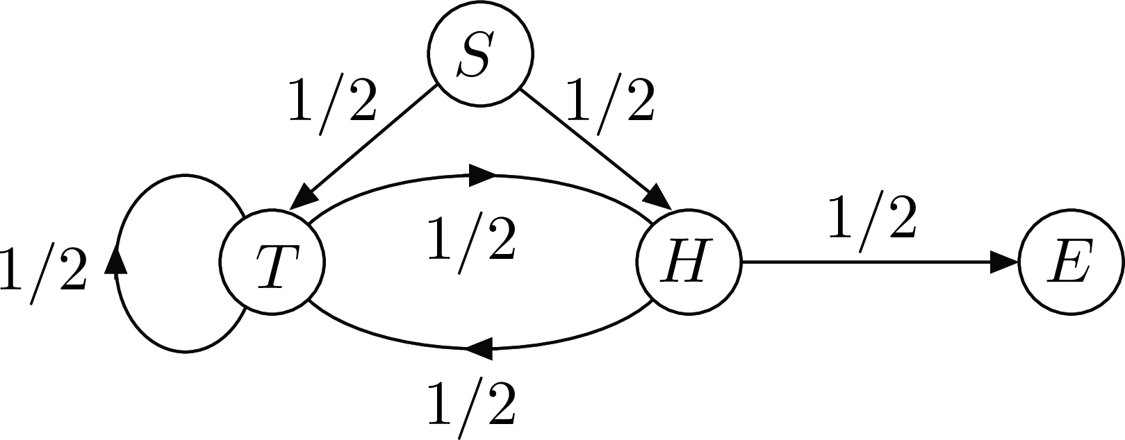
Figure 5: Flipping a fair coin until two heads in row.
Say that you flip a fair coin repeatedly until you get two heads in a row. How many times do you have to flip the coin, on average? Figure 5 shows a state transition diagram that corresponds to that situation. The Markov chain starts in state \(S\). The state is \(H\) or \(T\) if the last coin flip was \(H\) or \(T\), except that the state is \(E\) if the last two flips where heads. For \(i \in \{S, T, H, E\}\), let \(\beta(i)\) be the average number of steps until the Markov chain enters state \(E\). The first step equations are \[\begin{aligned} \beta(S) &= 1 + \frac{1}{2} \beta(T) + \frac{1}{2}\beta(H) \\ \beta(T) &= 1 + \frac{1}{2} \beta(T) + \frac{1}{2} \beta(H) \\ \beta(H) &= 1 + \frac{1}{2} \beta(T) + \frac{1}{2} \beta(E) \\ \beta(E) &= 0.\end{aligned}\] Solving, we find \[ \beta(S) = 6.\](13) (See the appendix for the calculations.)
Now assume you roll a balanced six-sided die until the sum of the last two rolls is \(8\). The Markov chain that corresponds to this situation has a start state \(S\), a state \(i\) for \(i \in \{1, 2, \ldots, 6\}\) that indicates the value of the last roll, and an end state \(E\) that the Markov chain enters when the sum of the last two rolls is \(8\). Thus, if the state of the Markov chain is \(5\) and if the next roll is \(2\), then the new state is \(2\). However, if the next roll is \(3\), then the Markov chain enters state \(E\). The first step equations for the average time \(\beta(i)\) it takes the Markov chain to enter state \(E\) are as follows: \[\begin{aligned} \beta(S) &= 1 + \sum_{i = 1}^6 \frac{1}{6} \beta(i) \\ \beta(i) &= 1 + \sum_{j \text{ s.t. } i + j \neq 8} \frac{1}{6} \beta(j).\end{aligned}\] Solving, we find \[ \beta(S) = 8.4.\](14) (See the appendix for the calculations.)
Consider now the \(20\)-rung ladder. A man starts on the ground. At each step, he moves up one rung with probability \(p\) and falls back to the ground otherwise. Let \(\beta(i)\) be the average number of steps needed to reach the top rung, starting from rung \(i \in \{0, 1, \ldots, 20\}\) where rung \(0\) refers to the ground. The first step equations are \[\begin{aligned} \beta(i) &= 1 + (1 - p)\beta(0) + p \beta(i + 1), i = 0, \ldots, 19\\ \beta(20) &= 0.\end{aligned}\] Solving, we find \[ \beta(0) = \frac{p^{-20} - 1}{1 - p}.\](15) (See the appendix for the calculations.) For instance, if \(p = 0.9\), then \(\beta(0) \approx 72\). Also, if \(p = 0.8\), then \(\beta(0) \approx 429\). The morale of the story is that you have to be careful on a ladder.
Assume we play a game of heads-or-tails with a coin such that \({\mathbb{P}}[H] = p\). For every heads, your fortune increases by \(1\) and for every tails, it decreases by \(1\). The initial fortune is \(m\). Let \(\beta(n)\) be the average time until the fortune reaches the value \(0\) or the value \(M\) where \(M > m\). The first step equations are \[\begin{aligned} \beta(n) &= 1 + (1 - p) \beta(n-1) + p \beta(n+1), \mbox{ for } n = 1, \ldots, M -1 \\ \beta(0) &= \beta(M) = 0.\end{aligned}\] Solving, we find \[ \beta(n) = n (1 - 2p)^{-1} - \frac{M(1 - 2p)^{-1}}{1 - \rho^M} (1 - \rho^n).\](16) (See the appendix for the calculations.)
Probability of \(A\) before \(B\)
Let \(X_n\) be a finite Markov chain with state space \({\cal X}\) and transition probability matrix \(P\). Let also \(A\) and \(B\) be two disjoint subsets of \({\cal X}\). We want to determine the probability \(\alpha(i)\) that, starting in state \(i\), the Markov chain enters one of the states in \(A\) before one of the states in \(B\).
The first step equations for \(\alpha(i)\) are \[\begin{aligned} \alpha(i) &= \sum_j P(i, j) \alpha(j), \forall i \notin A \cup B \\ \alpha(i) &= 1, \forall i \in A \\ \alpha(i) &= 0, \forall i \in B.\end{aligned}\]
To see why the first set of equations hold, we observe that the event that the Markov chain enters \(A\) before \(B\) starting from \(i\) is partitioned into the events that it does so by first moving to state \(j\), for all possible value of \(j\). Now, the probability that it enters \(A\) before \(B\) starting from \(i\) after moving first to \(j\) is the probability that it enters \(A\) before \(B\) starting from \(j\), because the Markov chain is amnesic. The second and third sets of equations are obvious.
As an illustration, consider again the game of heads and tails and let \(\alpha(n)\) be the probability that your fortune reaches \(M\) before \(0\) when starting from \(n\) with \(0 \leq n \leq M\). The first step equations are \[\begin{aligned} \alpha(n) &= (1 - p) \alpha(n-1) + p \alpha(n+1), 0 < n < M \\ \alpha(M) &= 1 \\ \alpha(0) &= 0.\end{aligned}\] Solving these equations, we find \[ \alpha(n) = \frac{1 - \rho^n}{1 - \rho^M}\](17) where \(\rho := (1 - p)p^{-1}\). (See the appendix for the calculations.) For instance, with \(p = 0.48\) and \(M = 100\), we find that \(\alpha(10) \approx 4 \times 10^{-4}\), which is sobering when contemplating a trip to Las Vegas. Note that for each gambler who plays this game, the Casino makes \(\$10.00\) with probability \(1 - 4 \times 10^{-4}\) and loses \(\$990.00\) with probability \(4 \times 10^{-4}\), so that the expected gain of the Casino per gambler is approximately \((1 - 4 \times 10^{-4}) \times \$10.00 - 4 \times 10^{-4} \times \$990.00 \approx \$9.60\). Observe that the probability of winning in one step is \(48\%\), so that if the gamble did bet everything on a single game and stopped after one step, the Casino would only make \(0.52 \times \$10.00 - 0.48 \times \$10.00 = \$0.40\) on average per gambler, instead of \(\$9.60\). The morale of the story is: don’t push your luck!
Appendix 1: Calculations
This section presents the details of the calculations of this note.
- Equation 3
By symmetry, we can write \[P^n = \begin{bmatrix} 1 - \alpha_n & \alpha_n \\ \alpha_n & 1 - \alpha_n \end{bmatrix} \] for some \(\alpha_n\) that we determine below. Note that \(\alpha_1 = a\). Also, \[P^{n+1} = \begin{bmatrix} 1 - \alpha_{n+1} & \alpha_{n+1} \\ \alpha_{n+1} & 1 - \alpha_{n+1} \end{bmatrix} = P P^n = \begin{bmatrix} 1 - a & a\\ a & 1 - a \end{bmatrix} \begin{bmatrix} 1 - \alpha_n & \alpha_n \\ \alpha_n & 1 - \alpha_n \end{bmatrix} .\] Consequently, by looking at component \((0, 1)\) of this product, \[\alpha_{n+1} = (1 - a) \alpha_n + a (1 - \alpha_n) = a + (1 - 2a) \alpha_n.\] Let us try a solution of the form \(\alpha_n = b + c \lambda^n\). We need \[\alpha_{n+1} = b + c \lambda^{n+1} = a + (1 - 2a) \alpha_n = a + (1 - 2a)[b + c \lambda^n] = a + (1 - 2a)b + (1 - 2a)c \lambda^n.\] Matching the terms, we see that this identity holds if \[b = a + (1 -2a)b \text{ and } \lambda = 1 - 2a.\] The first equation gives \(b = 1/2\). Hence, \(\alpha_n = 1/2 + c(1 - 2a)^n\). To find \(c\), we use the fact that \(\alpha_1 = a\), so that \(1/2 + c(1 - 2a) = a\), which yields \(c = - 1/2\).
Hence, \(\alpha_n = 1/2 - (1/2)(1 - 2a)^n\).
- Equation 5
The balance equations are \(\pi = \pi P\).
We know that the equations do not determine \(\pi\) uniquely. Let us choose arbitrarily \(\pi(A) = 1\). We then solve for the other components of \(\pi\) and we renormalize later. We can ignore any equation we choose. Let us ignore the first one. The new equations are \[\begin{bmatrix} \pi(B) & \pi(C) & \pi(D) & \pi(E) \end{bmatrix} = \begin{bmatrix} 1 & \pi(B) & \pi(C) & \pi(D) & \pi(E) \end{bmatrix} \begin{bmatrix} 1/2 & 0 & 1/2 & 0 \\ 0 & 1 & 0 & 0 \\ 0 & 0 & 0 & 0 \\ 1/3 & 0 & 0 & 1/3 \\ 1/2 & 1/2 & 0 & 0 \\ \end{bmatrix} .\] Equivalently, \[\begin{bmatrix} \pi(B) & \pi(C) & \pi(D) & \pi(E) \end{bmatrix} = \begin{bmatrix} 1/2 & 0 & 1/2 & 0 \end{bmatrix} + \begin{bmatrix} \pi(B) & \pi(C) & \pi(D) & \pi(E) \end{bmatrix} \begin{bmatrix} 0 & 1 & 0 & 0 \\ 0 & 0 & 0 & 0 \\ 1/3 & 0 & 0 & 1/3 \\ 1/2 & 1/2 & 0 & 0 \\ \end{bmatrix} .\] By inspection, we see that \(\pi(D) = 1/2\), then \(\pi(E) = (1/3) \pi(D) = 1/6\), then \(\pi(B) = 1/2 + (1/3) \pi(D) + (1/2) \pi(E) = 1/2 + 1/6 + 1/12 = 3/4\). Finally, \(\pi(C) = \pi(B) + (1/2) \pi(E) = 3/4 + 1/12 = 5/6.\) The components \(\pi(A) + \cdots + \pi(E)\) add up to \(1 + 3/4 + 5/6 + 1/2 + 1/6 = 39/12.\) To normalize, we multiply each component by \(12/39\) and we get \[\pi = \begin{bmatrix} 12/39 & 9/39 & 10/39 & 6/39 & 2/39 \end{bmatrix}.\]
We could have proceeded differently and observed that our identity implies that \[\begin{bmatrix} \pi(B) & \pi(C) & \pi(D) & \pi(E) \end{bmatrix} \begin{bmatrix} 1 & -1 & 0 & 0 \\ 0 & 1 & 0 & 0 \\ - 1/3 & 0 & 1 & - 1/3 \\ - 1/2 & -1/2 & 0 & 1 \\ \end{bmatrix} = \begin{bmatrix} 1/2 & 0 & 1/2 & 0\end{bmatrix} .\] Hence, \[\begin{bmatrix} \pi(B)& \pi(C)& \pi(D)& \pi(E)\end{bmatrix} = \begin{bmatrix}1/2& 0& 1/2& 0\end{bmatrix} \begin{bmatrix} 1 & -1 & 0 & 0 \\ 0 & 1 & 0 & 0 \\ - 1/3 & 0 & 1 & - 1/3 \\ - 1/2 & -1/2 & 0 & 1 \\ \end{bmatrix} ^{-1}.\] This procedure is a systematic way to solve the balance equations by computer.
- Equation 12
Using the third equation in the second, we find \(\beta(B) = 2 + \beta(A)\). The fourth equation then gives \(\beta(D) = 1 + (1/3) \beta(A) + (1/3)(2 + \beta(A)) = 5/3 + (2/3) \beta(A)\). The first equation then gives \(\beta(A) = 1 + (1/2)(2 + \beta(A)) + (1/2)[5/3 + (2/3)\beta(A)] = 17/6 + (5/6) \beta(A)\). Hence, \((1/6) \beta(A) = 17/6\), so that \(\beta(A) = 17\). Consequently, \(\beta(B) = 19\) and \(\beta(D) = 5/3 + 34/3 = 13\). Finally, \(\beta(C) = 18\).
- Equation 13
The last two equations give \(\beta(H) = 1 + (1/2)\beta(T)\). If we substitute this expression in the second equation, we get \(\beta(T) = 1 + (1/2) \beta(T) + (1/2)[1 + (1/2) \beta(T)]\), or \(\beta(T) = 3/2 + (3/4) \beta(T)\). Hence, \(\beta(T) = 6\). Consequently, \(\beta(H) = 1 + (1/2)6 = 4\). Finally, \(\beta(S) = 1 + (1/2)6 + (1/2)4 = 6\).
- Equation 14
Let us write the equations explicitly: \[\begin{aligned} \beta(S) &= 1 + \frac{1}{6} [\beta(1) + \beta(2) + \beta(3) + \beta(4) + \beta(5) + \beta(6)] \\ \beta(1) &= 1 + \frac{1}{6} [\beta(1) + \beta(2) + \beta(3) + \beta(4) + \beta(5) + \beta(6)] \\ \beta(2) &= 1 + \frac{1}{6} [\beta(1) + \beta(2) + \beta(3) + \beta(4) + \beta(5)] \\ \beta(3) &= 1 + \frac{1}{6} [\beta(1) + \beta(2) + \beta(3) + \beta(4) + \beta(6)] \\ \beta(4) &= 1 + \frac{1}{6} [\beta(1) + \beta(2) + \beta(3) + \beta(5) + \beta(6)] \\ \beta(5) &= 1 + \frac{1}{6} [\beta(1) + \beta(2) + \beta(4) + \beta(5) + \beta(6)] \\ \beta(6) &= 1 + \frac{1}{6} [\beta(1) + \beta(3) + \beta(4) + \beta(5) + \beta(6)].\end{aligned}\] These equations are symmetric in \(\beta(2), \ldots, \beta(6)\). Let then \(\gamma = \beta(2) = \cdots = \beta(6)\). Also, \(\beta(1) = \beta(S)\). Thus, we can write these equations as \[\begin{aligned} \beta(S) &= 1 + \frac{1}{6}[\beta(S) + 5 \gamma] = 1 + \frac{1}{6} \beta(S) + \frac{5}{6} \gamma \\ \gamma &= 1 + \frac{1}{6}[ \beta(S) + 4 \gamma] = 1 + \frac{1}{6} \beta(S) + \frac{2}{3} \gamma.\end{aligned}\] The first equation gives \[\beta(S) = \frac{6}{5} + \gamma.\] The second yields \[\gamma = 3 + \frac{1}{2} \beta(S).\] Substituting the next to last identity into the last one gives \[\gamma = 3 + \frac{1}{2}\left[\frac{6}{5} + \gamma\right] = \frac{18}{5} + \frac{1}{2} \gamma.\] Hence, \[\gamma = \frac{36}{5}\] and, consequently, \[\beta(S) = \frac{6}{5} + \frac{36}{5} = \frac{42}{5} = 8.4.\]
- Equation 15
Let us look for a solution of the form \(\beta(i) = a + b \lambda^i\). Then \[a + b \lambda^i = 1 + (1 - p) (a + b) + p [a + b \lambda^{i+1}] = 1 + (1 - p) (a + b) + pa + bp \lambda^{i +1}.\] This identity holds if \[a = 1 + (1 - p)(a + b) + pa \text{ and } \lambda = p^{-1},\] i.e., \[b = - (1 - p)^{-1} \text{ and } \lambda = p^{-1}.\] Then, \[\beta(i) = a - (1 - p)^{-1} p^{-i}.\] Since \(\beta(20) = 0\), we need \[0 = a - (1 - p)^{-1} p^{- 20},\] so that \(a = (1 - p)^{-1} p^{- 20}\) and \[\beta(i) = (1 - p)^{-1} p^{- 20} - (1 - p)^{-1} p^{-i} = \frac{p^{-20} - p^{-i}}{1 - p}.\]
- Equation 16
Let us make a little detour into the solution of such difference equations. Assume you have a function \(g(n)\) such that \[g(n) = 1 + (1 - p) g(n-1) + pg(n - 1)\] and two functions \(\beta(n) = h(n)\) and \(\beta(n) = k(n)\) such that \[\beta(n) = (1 - p) \beta(n-1) + p \beta(n+1).\] Then, for any two constants \(a\) and \(b\), we note that \(\beta(n) := g(n) + a \cdot h(n) + b \cdot k(n)\) satisfies \[\beta(n) = 1 + (1 - p) \beta(n-1) + p \beta(n+1).\] We can then choose the two constants \(a\) and \(b\) to make sure that \(0 = \beta(0) = \beta(M)\).
To find \(g(n)\), we try \(g(n) = \alpha n\). We need \[\alpha n = 1 + (1 - p) \alpha (n - 1) + p \alpha (n + 1) = 1 + \alpha n - (1 - p) \alpha + p \alpha = \alpha n + 1 - \alpha + 2p \alpha.\] Thus, we need \(1 - \alpha + 2 p \alpha = 0\), i.e., \(\alpha = (1 - 2p)^{-1}\).
To find solutions to \(\beta(n) = (1 - p) \beta(n-1) + p \beta(n+1)\), we try \(\beta(n) = \lambda^n\). Then, \[\lambda^n = (1 - p) \lambda^{n-1} + p \lambda^{n+1}.\] With \(n = 1\), this gives \[\lambda = (1 - p) + p \lambda^2.\] Hence, \[p \lambda^2 - \lambda + (1 - p) = 0.\] The solutions of this quadratic equation are \[\lambda = \frac{ 1 \pm \sqrt{1 - 4p(1 - p)} }{2p} = \frac{1 \pm (1 - 2p)}{2p} = 1 \text{ and } \rho := (1 - p)p^{-1}.\] Thus, we find two such solutions that correspond to these two values of \(\lambda\): \[h(n) := 1 \mbox{ and } k(n) := \rho^n.\] We now choose the two parameters \(a\) and \(b\) so that \(\beta(n) = g(n) + a h(n) + b k(n)\) satisfies the two conditions \(\beta(0) = \beta(M) = 0\). This should give us two equations in the two unknowns \(a\) and \(b\).
These equations are \[0 = \beta(0) = g(0) + a h(0) + b k(0) = 0 + a \times 1 + b \times 1 = a + b\] and \[0 = \beta(M) = g(M) + a h(M) + b k(m) = M (1 - 2p)^{-1} + a \times 1 + b \times \rho^M.\] The first equation gives \(b = - a\), so that the second implies \[0 = M(1 - 2p)^{-1} + a(1 - \rho^M).\] Hence, \[a = - \frac{M(1 - 2p)^{-1}}{1 - \rho^M}.\] Finally, \[\beta(n) = n (1 - 2p)^{-1} - \frac{M(1 - 2p)^{-1}}{1 - \rho^M} (1 - \rho^n).\]
- Equation 17
In the calculation of Equation 16, we found two solutions to Equation 17: \[\alpha(n) = 1 \text{ and } \alpha(n) = \rho^n\] with \(\rho = (1 - p)p^{-1}\). Hence, for any two constants \(a\) and \(b\), a solution is \(\alpha(n) = a + b \rho^n\). We now choose \(a\) and \(b\) so that \(\alpha(0) = 0\) and \(\alpha(M) = 1\). That is, \[0 = a + b \text{ and } 1 = a + b \rho^M.\] Thus, \(b = - a\) and \[1 = a(1 - \rho^M), \text{ i.e., } a = (1 - \rho^M)^{-1}.\] Hence, \[\alpha(n) = a + b \rho^n = a(1 - \rho^n) = \frac{1 - \rho^n}{1 - \rho^M}.\]
Appendix 2: Some Proofs
Proof Sketch of Theorem 3. A formal proof of Theorem 3 is a bit complicated. However, we can sketch the argument to justify the result.
First let us explain why Equation 8 implies that the invariant distribution is unique. Assume that \(\nu = \{\nu(i), i \in {\cal X}\}\) is an invariant distribution and choose \(\pi_0 = \nu\). Then \({\mathbb{P}}[X_n = i] = \nu(i)\) for all \(n \geq 0\). Call \(Y_n\) the fraction in Equation 8. Note that \({\mathbb{E}}[Y_n] = \nu(i)\) for all \(n\), because \({\mathbb{E}}[1\{X_m = i\}] = {\mathbb{P}}[X_m = i] = \nu(i)\). Now, Equation 8 says that \(Y_n \to \pi(i)\). We claim that this implies that \({\mathbb{E}}[Y_n] \to \pi(i)\), so that \(\nu(i) \to \pi(i)\), which implies that \(\nu(i) = \pi(i)\). To prove the claim, we use the fact that \(Y_n \to \pi(i)\) implies that, for any \(\epsilon > 0\), there is some \(n\) large enough so that \({\mathbb{P}}[|Y_m - \pi(i)| \leq \epsilon] \geq 1 - \epsilon\) for all \(m \geq n\). But then, because \(Y_m \in [0, 1]\), we see that \({\mathbb{E}}[|Y_m - \pi(i)|] \leq \epsilon(1 - \epsilon) + \epsilon\), so that \(|{\mathbb{E}}[Y_m] - \pi(i)| \leq {\mathbb{E}}[|Y_m - \pi(i)|] \leq 2 \epsilon\). This shows that \({\mathbb{E}}[Y_m] \to \pi(i)\).
The second step is to note that all the states must be recurrent, which means that the Markov chain visits them infinitely often. Indeed, at least one state, say state \(i\), must be recurrent since there are only finitely many states. Consider any other state \(j\). Every time that the Markov chain visits \(i\), it has a positive probability \(p\) of visiting \(j\) before coming back to \(i\). Otherwise, the Markov chain would never visit \(j\) when starting from \(i\), which would contradict its irreducibility. Since the Markov chain visits \(i\) infinitely often, it also must visit \(j\) infinitely often, in the same way that if you flip a coin with \({\mathbb{P}}[H] = p > 0\) forever, you must see an infinite number of \(H\)s.
The third step is to observe that the times \(T(i, 1), T(i, 2), \ldots\) between successive visits to one state \(i\) are independent and identically distributed, because the motion of the Markov chain starts afresh whenever it enters state \(i\). By the law of large number, \((T(i, 1) + \cdots + T(i, n))/n \to {\mathbb{E}}[T(i, 1)]\) as \(n \to \infty\). Hence, \(n/(T(i, 1) + \cdots + T(i, n)) \to \pi(i) := 1/{\mathbb{E}}[T(i, 1)]\). That is, the rate of visits of state \(i\) is \(\pi(i)\).
The fourth step is to show that \(\pi(i) > 0\) for all \(i\). Indeed, \(\pi(i) > 0\) for at least one state \(i\), otherwise the rate of visits of all the states would be zero, which is not possible since these rates of visit add up to one. Also, if the Markov chain visits state \(i\) with rate \(\pi(i) > 0\), then it visits state \(j\) with at least rate \(\pi(i)p > 0\) because it visits \(j\) with probability \(p\) between two visits to \(i\). Hence, \(\pi(j) > 0\) for all \(j\).
The fifth step is to show that \(\pi(i)\) satisfies the balance equations. We saw that, during a large number \(n\) of steps, the Markov chain visits state \(j\) approximately \(n \pi(j)\) times. Consider then a given state \(i\). Since that state is visited with probability \(P(j, i)\) after each visit to state \(j\), state \(i\) should be visited approximately \(n \pi(j) P(j, i)\) times immediately after the \(n \pi(j)\) visits to state \(j\). If we sum over all the states \(j\), we see that state \(i\) should be visited approximately \(n \sum_j \pi(j) P(j, i)\) times over \(n\) steps. But we know that this number of visits is approximately \(n \pi(i)\). Hence, it must be that \(n \sum_j \pi(j)P(j, i) \approx n \pi(i)\), i.e., that \(\pi(i) = \sum_j \pi(j) P(j, i)\). These are the balance equations. \(\square\)
Proof of Theorem 4. We give the proof in the aperiodic case, i.e., when there is some state \(i\) such that \(d(i) = 1\).
Define \(S(i) = \{n > 0 \mid P^n(i, i) > 0\}\). We fist show that there is some integer \(n(i)\) so that \(n \in S(i)\) if \(n \geq n(i)\). Note that if \(\gcd(S(i)) = 1\), then there must be \(a, b \in S(i)\) with \(\gcd\{a, b\} = 1\). Using Euclid’s extended GCD algorithm, we find integers \(m\) and \(n\) so that \(m a + n b = \gcd\{a, b\} = 1\). Let \(m^+ = \max\{0, m\}, n^+ = \max\{0, n\}, m^- = m + m^+, n^- = n + n^+\). Then \((m^+ - m^-)a + (n^+ - n^-)b = 1\) and we note that \(k := m^- a + n^- b\) and \(k+1 = m^+a + n^+ b\) are both in \(S(i)\). Now, if \(n \geq k^2\), then one can write \(n = ak + b\) for some \(b \in \{0, 1, \ldots, k -1\}\) and some \(a > k - 1\). But then \[n = ak + b = (a - b)k + b(k+1) \in S(i),\] since both \(k\) and \(k + 1\) are in \(S(i)\). Thus, any \(n \geq n(i) = k^2\) is such that \(n \in S(i)\).
Next we show that \(d(j) = 1\) for every state \(j\). Since it is irreducible, the Markov chain can go from \(j\) to \(i\) is some \(a\) steps and from \(i\) to \(j\) in some \(b\) steps. But the Markov chain can go from \(i\) to \(i\) in \(n(i)\) or in \(n(i) + 1\) steps. Consequently, the Markov chain can go from \(j\) to \(j\) in \(a + n(i) + b\) steps and also in \(a + n(i) + 1 + b\) steps by going from \(j\) to \(i\) in \(a\) steps, then from \(i\) to \(i\) in \(n(i)\) or \(n(i) + 1\) steps, then from \(i\) to \(j\) in \(b\) steps. Hence, \(\{n > 0 \mid P^n(j, j) > 0\}\) contains two consecutive integers \(a + n(i) + b\) and \(a + n(i) + 1 + b\), so that its g.c.d. must be equal to one. Thus, \(d(j) = 1\) for every state \(j\).
Let us now fix a state \(i\) arbitrarily. The claim is that there is some integer \(k\) such that the Markov chain can go from any state \(j\) to state \(i\) in \(k\) steps. To see this, using the irreducibility of the Markov chain, we know that for every \(j\) there is some integer \(n(j, i)\) so that the Markov chain can go from \(j\) to \(i\) in \(n(j, i)\) steps. But then, the Markov chain can go from \(j\) to \(i\) in \(n + n(j, i)\) steps for any \(n \geq n(j)\). Indeed, the Markov chain can go first from \(j\) to \(j\) in \(n\) steps, then from \(j\) to \(i\) in \(n(j, i)\) steps. Thus, the Markov chain can go from \(j\) to \(i\) in \(n\) steps, for any \(n \geq n(j) + n(j, i)\). We then let \(k = \max_j \{n(j) + n(j, i)\}\).
Next, consider two independent copies \(X_n\) and \(Z_n\) of the Markov chain with transition matrix \(P\). Markov chain \(X_n\) starts with the invariant distribution \(\pi\). Markov chain \(Z_n\) starts with an arbitrary initial distribution \(\pi_0\). Define state \(i\) and the integer \(k\) as in the previous paragraph. There is some positive probability \(p\) that the two Markov chains both are in state \(i\) after \(k\) steps. If not, there is again a probability \(p\) that they are both in state \(i\) after \(k\) more steps, and so on. Thus, if we designate by \(\tau\) the first time that the two Markov chains meet, i.e., \(\tau = \min \{n \geq 0 \mid X_n = Z_n\}\), we see that \({\mathbb{P}}[\tau > km] \leq (1 - p)^m\) for \(m = 1, 2, \ldots\). Now, define the Markov chain \(Y_n\) so that \(Y_n = Z_n\) for \(n < \tau\) and \(Y_n = X_n\) for \(n \geq \tau\). In words, the Markov chain starts like \(Z_n\), but it sticks to \(X_n\) once \(X_n = Z_n\). This Markov chain \(Y_n\) still has transition matrix \(P\) and its initial distribution is \(\pi_0\). Note that \({\mathbb{P}}[X_n \neq Y_n] = {\mathbb{P}}[\tau > n] \to 0\) as \(n \to \infty\). Hence, \[|{\mathbb{P}}[X_n = i] - {\mathbb{P}}[Y_n = i]| \leq {\mathbb{P}}[X_n \neq Y_n] \to 0, \text{ as } n \to \infty.\] But \({\mathbb{P}}[X_n = i] = \pi(i)\) for all \(n\) since \(X_n\) starts with the invariant distribution \(\pi\). We conclude that \({\mathbb{P}}[Y_n = i] \to \pi(i)\) as \(n \to \infty\). \(\square\)
The observant reader will have noticed that the LHS of Equation 8 is a random variable, and the RHS of Equation 8 is a constant, so Equation 8 does not make sense, strictly speaking! In fact, when discussing random variables, there are numerous ways to formalize the notion of convergence. One of them is convergence in probability, which we have already encountered when we introduced the weak law of large numbers: \[ \lim_{n\to\infty} {\mathbb{P}}\!\left(\left| \frac{1}{n} \sum_{m=0}^{n-1} 1\{X_m = i\} - \pi(i) \right| > \varepsilon\right) = 0, \qquad \forall \varepsilon > 0. \](6) Another form of convergence is convergence with probability \(1\): \[ {\mathbb{P}}\!\left(\lim_{n\to\infty} \frac{1}{n} \sum_{m=0}^{n-1} 1\{X_m = i\} = \pi(i)\right) = 1. \](7) It turns out that Equation 7 implies Equation 6 and in this case, both types of convergence occur. Furthermore, since the LHS of Equation 8 is bounded, we also have convergence of expected value: \[ \lim_{n\to\infty} \frac{1}{n} \sum_{m=0}^{n-1} {\mathbb{P}}(X_m = i) = \pi(i). \]↩